Transformers and Self Attention

Before we dive into the deep end, I realized something: I completely forgot to introduce myself in Part 1! Hi, I’m Kshayik Doshi, and I’m weirdly passionate about computers. I’m currently pursuing Computer Engineering at DJ Sanghvi in my final year. I spend most of my time living in two different worlds—building low-level systems in C++ and hacking together AI products and agentic pipelines. Now that we’ve officially met, let's get right back to business.

Where We Left Off (The Quick Recap)

In Part 1, we laid down the ground rules for how language models operate at a foundational level:

• Tokens & Encoding: How raw text gets mapped into numerical IDs and dense vectors.
• Chunks & Context: How splitting text into fixed block_size chunks teaches the model multiple next-token prediction lessons in a single pass.
• Tensors ($[B \times T \times C]$): The 3D tensor shape flowing through the network—Batch Size ($B$), Sequence Length ($T$), and Embedding Dimension / Channels ($C$).
• Loss & Generation: How Cross-Entropy loss scores predictions and how autoregressive generation loops one token at a time.

Why We Needed GPT in the First Place

At the end of Part 1, we ran text generation on our baseline model and got absolute Shakespearean gibberish.

Why? Because what we had built was essentially a glorified Bigram model. The prediction for the next character was happening almost purely through a local lookup table based on the current character alone. It had no real memory and zero contextual awareness.

Historically, researchers tried solving this context problem using RNNs (Recurrent Neural Networks) and LSTMs (Long Short-Term Memory Networks) by passing a "hidden state" sequentially from one token to the next. But they hit two major brick walls:

1. The Sequential Bottleneck: Token #50 could not be processed until Token #49 was finished. Because processing was strictly sequential, it was impossible to parallelize training on modern hardware.
2. Vanishing Context: Passing information down a sequential chain is like a game of telephone. By the time the hidden state reached the end of a sentence, information from the beginning was diluted or completely forgotten.

We needed a way for every token in the context window to directly talk to every other token at the exact same time, fully parallelized.

Enter the Transformer architecture and the breakthrough mechanism from Attention Is All You Need: Self-Attention.

Static vs. Contextual Embeddings

Before diving into the attention mechanics, we need to look closer at embeddings. Google defines embeddings as:

"Embeddings are numerical representations of real-world data, such as words, images, or audio, translated into lists of floating-point numbers. By plotting these numbers in a multi-dimensional mathematical space, AI models group similar concepts close together, allowing algorithms to easily 'understand' meaning, context, and relationship."

I want you to pay close attention to that phrase: grouping similar concepts together.

When a model looks up an embedding vector for a token in a lookup table, that vector is static. The string "Apple" gets assigned the exact same array of floating-point numbers regardless of where it appears:

• Sentence A: "I bought an Apple phone yesterday." $\longrightarrow$ Refers to the tech company.
• Sentence B: "I bought an apple at the market." $\longrightarrow$ Refers to the fruit.

The token string "Apple" is identical in both cases, but its meaning changes completely based on surrounding context. Static embeddings alone cannot capture this distinction.

Self-Attention is the engine that converts static semantic embeddings into contextual embeddings. It allows tokens to look at surrounding words and dynamically update their representations accordingly.

Dissecting Self-Attention & The QKV Engine

So, what exactly is Self-Attention?

Self-Attention is a mechanism that enables models to understand context by relating different words within a sequence to one another.

Mathematically, it is defined by the iconic equation:

$$\text{Attention}(Q, K, V) = \text{softmax}\left(\frac{QK^T}{\sqrt{d_k}}\right)V$$

Okay, now is the time to grab a book and pen and actually write this down to understand it! To make tokens communicate, the Transformer assigns three distinct roles to every single token vector inside the $[B \times T \times C]$ tensor we discussed earlier:

• Query ($Q$): "What am I looking for?" (The question token $i$ asks).
• Key ($K$): "What information do I contain?" (The label token $j$ advertises).
• Value ($V$): "What actual content do I pass along if we match?" (The raw representation token $j$ shares).

(Fun side note: when people talk about the KV Cache during LLM inference, it's literally these exact Key and Value vectors being stored in memory so we don't recompute them for past tokens!)

Connecting $Q, K, V$ to the Tensor $[B \times T \times C]$

Remember the channel dimension $C$ from our $[B \times T \times C]$ tensor? That row along $C$ is originally just the static embedding vector from our lookup table.

To transform it, we multiply our tensor by three learnable linear projection matrices ($W_Q, W_K, W_V$). Now, every token vector has its own Query, Key, and Value vectors.

When it comes to being computational beasts, we handle all of this simultaneously using matrix multiplication:

1. Calculating Attention Scores ($Q \cdot K^T$): We multiply the Query matrix of all tokens by the transposed Key matrix of all tokens. This produces a $[T \times T]$ score matrix where entry $(i, j)$ represents how much Token $i$ matches Token $j$.
2. Scaling by $\sqrt{d_k}$: Why do we divide by $\sqrt{d_k}$? When the key dimension $d_k$ is large, dot products get huge. Passing huge numbers into Softmax causes it to saturate (returning $1.0$ for the highest score and near $0.0$ for everything else), which leads to vanishing gradients during training. Scaling by $\sqrt{d_k}$ keeps the scores at a manageable scale.
3. Softmax Normalization: We apply Softmax row by row so the scores turn into probabilities that sum to $1.0$.
4. Weighted Sum ($\text{Softmax} \cdot V$): Finally, we multiply these attention weights by the Value matrix $V$.

Each token takes a weighted proportion of every other token's Value vector and sums them up. The result? The static embedding along $C$ is now updated into a brand-new contextual embedding!

Causal Self-Attention (Masking)

There's one crucial rule in GPT: generation happens left-to-right.

When training on a sequence like "I love eating pizza", Token #2 ("eating") should only use context from "I", "love", and "eating". If it's allowed to attend to Token #3 ("pizza"), it will cheat by peeping into the future!

To prevent this, we apply Causal Masking. Before applying Softmax, we take all upper-triangular positions in the $[T \times T]$ attention score matrix (where token $j > i$) and force their values to $-\infty$ (negative infinity):

$$\text{Masked Score}_{i,j} = -\infty \quad \text{for } j > i$$

Because $e^{-\infty} = 0$, applying Softmax turns all future attention weights into an exact 0%. The model is completely blinded to future tokens during training!

Multi-Head Attention (MHA)

A single attention mechanism (one "head") can usually only focus on one type of relationship at a time—for example, matching verbs to their subjects. But language requires tracking multiple relationships simultaneously:

• Syntax and grammar rules
• Noun-pronoun relationships across long distances
• Semantic topic similarity

Instead of running one massive attention operation over the full dimension $C$, Multi-Head Attention (MHA) splits the embedding dimension $C$ into $h$ smaller sub-dimensions ($d_k = C / h$).

For instance, in GPT-2 Small:

• Embedding Dimension $C = 768$
• Number of Heads $h = 12$
• Head Dimension $d_k = 768 / 12 = 64$

Each head runs scaled causal self-attention independently in its own 64-dimensional subspace. The outputs from all 12 heads are concatenated back into a 768-dimensional tensor and multiplied by an output projection matrix $W_O$.

If you're a visual learner, check out this excellent resource: How Attention Mechanism Works in Transformer Architecture.

Feed-Forward Network (FFN): Token-Level Processing

If Self-Attention is all about communication (tokens exchanging information across the sequence), the Feed-Forward Network is where each token gets to do some individual thinking.

Once attention finishes gathering context, every token vector is passed through a position-wise Feed-Forward Network independently.

What Does "Position-Wise" Mean?

It means this exact same network is applied to every single token independently and identically. Token #1 goes through the FFN without knowing or caring about what Token #2 is doing in its FFN pass.

The Architecture: Expand, Activate, Project

Mathematically, the FFN consists of two linear transformations with a non-linear activation function in between:

$$\text{FFN}(x) = \max(0, x W_1 + b_1) W_2 + b_2$$

1. Linear Layer 1 ($x W_1 + b_1$): Projects the token from its original embedding dimension $C$ into a higher-dimensional space (typically $4 \times C$). For instance, an input dimension of $512$ gets blown up to $2048$ hidden units (or $768 \to 3072$ in GPT-2 Small).
2. Activation Function ($\text{ReLU} / \text{GELU}$): Applies a non-linear activation like ReLU ($\text{ReLU}(x) = \max(0, x)$) or GELU (used in modern GPT models). Without non-linearity, two back-to-back linear layers would just collapse into a single matrix multiplication!
3. Linear Layer 2 ($(\dots) W_2 + b_2$): Projects the vector back down from $4C$ to the original embedding dimension $C$ ($2048 \to 512$).

Expanding features into a higher-dimensional space gives the network scratchpad memory to process complex feature combinations before compressing that insight back into the standard channel vector.

The Glue: Add & Norm (LayerNorm, Residuals & Dropout)

To keep activations stable and prevent gradients from vanishing or exploding as we stack deeper layers, three critical components glue the Transformer together:

1. Residual Connections (Add)

A Residual Connection adds the unmodified input of a layer directly to its output:

$$\text{Output} = x + \text{SubLayer}(x)$$

This creates a "gradient highway." During backpropagation, gradients flow backwards through the addition operator unimpeded, allowing us to train deep networks without signal decay.

2. Layer Normalization (Norm)

Unlike Batch Normalization, LayerNorm calculates the mean $\mu$ and variance $\sigma^2$ across the channel features $C$ for each token independently:

$$\mu = \frac{1}{C} \sum_{i=1}^{C} x_i, \quad \sigma^2 = \frac{1}{C} \sum_{i=1}^{C} (x_i - \mu)^2$$ $$\text{LayerNorm}(x) = \frac{x - \mu}{\sqrt{\sigma^2 + \epsilon}} \cdot \gamma + \beta$$

Where $\gamma$ and $\beta$ are learnable scale/shift parameters, and $\epsilon$ prevents division by zero.

3. Dropout

During training, Dropout randomly zeros out a percentage of activations (typically 10%) at the end of sub-layers to prevent overfitting. During generation/inference, dropout is disabled.

Putting It All Together: The GPT-2 Decoder Block

Combining everything we've built, a single GPT-2 Transformer Block looks like this:

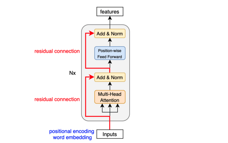
This single block is repeated $N$ times (e.g., $N=12$ layers in GPT-2 Small). After the final block, the tensor goes through a final LayerNorm, multiplied by the Linear LM Head to get logits over our vocabulary, and sampled to generate the next token.

Conclusion

This marks the end of our complete theory phase! Every piece of the Transformer exists for a logical reason:

• Tokenization & Embeddings convert language into numbers and dense vectors.
• Self-Attention gives words context by letting tokens talk to each other.
• Causal Masking stops the model from peeping into the future.
• Multi-Head Attention tracks multiple language relationships in parallel.
• Feed-Forward Networks give tokens space to process information individually.
• Residuals & LayerNorm keep deep network training stable.

The next step is to stop reading math and actually build one. In Part 3/5, the systems engineer in me takes over. We will write a complete, naive implementation of GPT from scratch in Modern C++, focusing purely on mathematical correctness before we start benchmarking and optimizing for hardware performance.

In the next part, we'll finally open the transformer itself and see why attention changed modern AI.