Going Full GPU

If you've made it this far, congrats cuh this the final stretch. We started by teaching a tiny model to predict the next token, then opened up the Transformer and understood what was actually happening inside attention. In Part 3, we finally took all of that theory and built the whole thing in C++.

Then came optimization. We flattened our tensors, fixed our memory access patterns, squeezed more work out of the CPU with AVX2 and FMA, and threw OpenMP at the parts that could run in parallel. None of that changed the math — we just made the CPU work a lot harder for us. And it worked.

But we've reached the point where optimization alone isn't going to save us.

Our tiny model can still run inference on a CPU without much drama. Training it is another story. Scale the model up, increase the context, increase the number of parameters, and suddenly the amount of computation becomes absolutely ridiculous.

And the funny part? We've spent the entire series writing code for CPUs. Now we're going to write code for something completely different.

Almost every piece of code I've written in my life has ultimately been running on a CPU. This time, we're moving to a machine built for doing thousands of things at once. We're going full GPU.

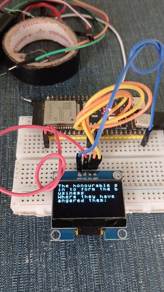
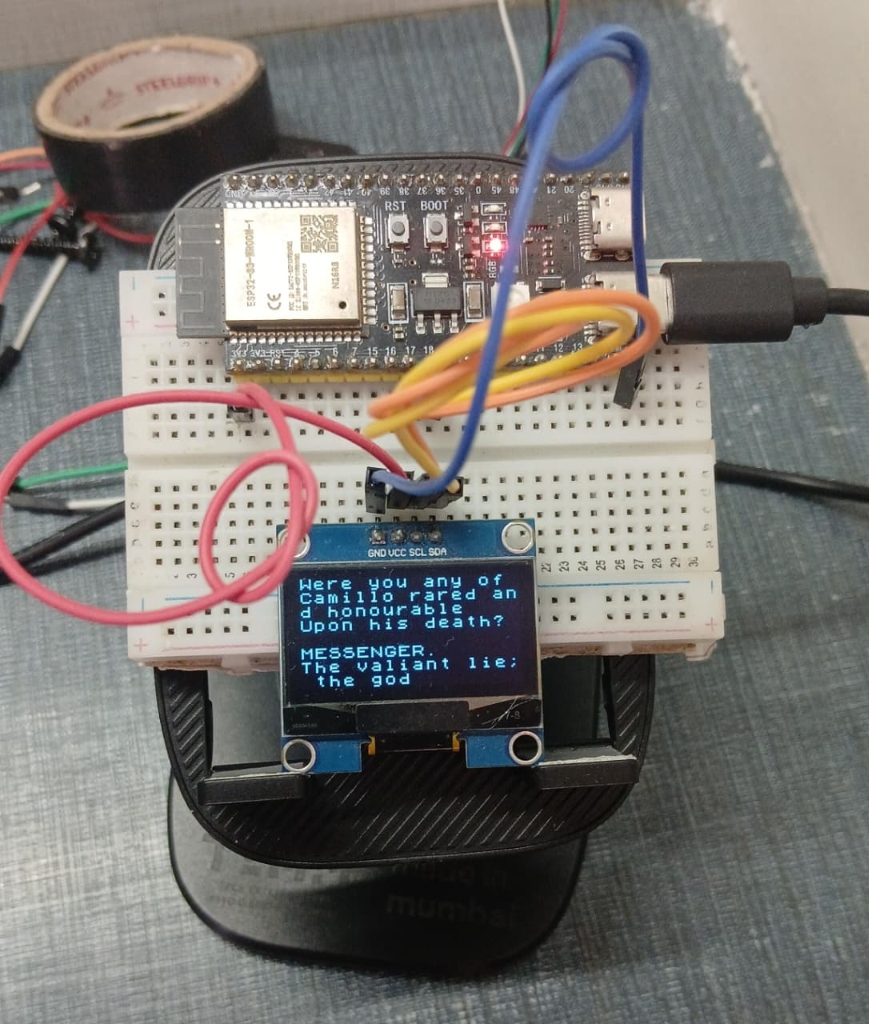
And stay till the end, because after all this talk about GPUs, CUDA, memory bandwidth and thousands of parallel threads, we're going to see just how much we can push this little model. We’re putting it on an ESP32 — and letting it mog basically every microcontroller whose only fault was to exist.

Why We Need GPUs

Why did our CPU start choking the moment we tried to push training harder? To understand that, we need to look at what CPUs and GPUs were actually built to do.

The CPU: The Low-Latency Brain

Think of a CPU core as an Olympic sprinter with a PhD. It’s built for complex, unpredictable work—branches, OS tasks, pointer-heavy code, and anything where each step depends on the last. That’s why CPUs invest heavily in a few powerful cores with features like branch prediction and large caches to reduce latency. But there are only a few of these cores.

The GPU: The Parallel Army

GPUs are built for a different world. If you’re rendering millions of pixels, each pixel can be computed independently. So instead of doing them one by one, why not do them all at once? That’s the GPU philosophy: trade complexity for massive parallelism. It’s not about making one operation faster—it’s about doing thousands at the same time. And that’s exactly what Transformers need.

Why Transformers and GPUs Fit So Well

Transformers rely heavily on matrix multiplications. This involves a huge number of independent multiply-accumulate operations. Each output element can be computed without waiting for others, making it ideal for parallel hardware. So the math didn’t change. We just moved it onto hardware designed to do many simple operations in parallel.

Speaking to the Metal: What is CUDA?

Back in the day, if you wanted to make a GPU do general math, you had to trick it into thinking your numbers were video game pixels. You literally had to disguise matrix multiplication as rendering a 3D polygon. Then NVIDIA released CUDA (Compute Unified Device Architecture). CUDA lets us bypass all that graphic abstraction and write C++ directly for GPU hardware. Instead of writing shader code, we write functions called kernels. A kernel is just regular C++ code that you write for one single thread, but tell the GPU to run on thousands of threads at the exact same time.

Two Separate Worlds: Host vs. Device

Before writing a single kernel, you have to understand the physical reality of your machine: your CPU and GPU do not share memory.

In CUDA terms:

• Host: Your CPU and system RAM.
• Device: Your GPU and its dedicated VRAM.

They sit on completely different physical boards connected by the PCIe slot on your motherboard. Compared to the speed of GPU memory, the PCIe bus is like a congested single-lane highway. Allocating memory on the GPU (cudaMalloc) and copying data across that bus (cudaMemcpy) is slow.

If you copy your tensors back to the CPU after every single matrix multiplication just to check on them, your GPU spends 95% of its time sitting idle, waiting on the PCIe bus.
The golden rule of GPU programming is simple:

"Send the data over once, keep everything inside VRAM for the entire forward pass, and only copy the final predicted tokens back to the CPU at the very end."

Memory Bandwidth vs. Compute Throughput (The FLOPS Trap)

But here’s the catch that catches most beginners off guard: a GPU's advertised FLOPS only tell half the story. You can have hundreds of teraflops of theoretical compute, but if your arithmetic execution units are constantly starved waiting for data to crawl in from VRAM, that horsepower is completely wasted. Just like our CPU optimizations in Part 3, high-performance GPU programming is all about memory traffic: maximizing arithmetic intensity, reusing data inside fast registers and on-chip __shared__ memory, and ensuring memory accesses stay aligned so the hardware stays continuously fed.

The Parallel Hierarchy: Threads, Blocks, and Grids

On the CPU, our mental model was a simple for loop:

// CPU Mindset: Walk through items one by one (or 8 at a time with SIMD)
for (int i = 0; i < N; ++i) {
    out[i] = gelu(in[i]);
}

On the GPU, we throw away the outer loop entirely. Instead of one core looping $N$ times, we launch $N$ threads simultaneously. Every thread runs the exact same code on its own piece of data. To organize this massive army, CUDA groups threads into a simple hierarchy:

• Thread: The individual worker computing one single value.
• Block: A group of threads (usually 128, 256, or 512). Threads inside the same block run on the same core cluster and can talk to each other through ultra-fast shared memory.
• Grid: The collection of all blocks launched to solve the entire problem.

Finding Your Seat in the Stadium

If you spawn 50,000 threads simultaneously, how does a specific thread know which array element belongs to it? Think of it like finding your assigned seat in a stadium. You need to know your Row (Block ID), the Row Size (Block Dimension), and your Seat Number (Thread ID):

In code, a CUDA kernel looks surprisingly simple:

// __global__ tells the compiler: "This runs on the GPU, called by the CPU"
__global__ void gelu_kernel(float* out, const float* in, int N) {
    // 1. Calculate unique global thread index
    int idx = blockIdx.x * blockDim.x + threadIdx.x;

    // 2. Boundary check (make sure extra threads don't read past the array)
    if (idx < N) {
        float x = in[idx];
        out[idx] = 0.5f * x * (1.0f + tanhf(0.7978845608f * (x + 0.044715f * x * x * x)));
    }
}

And to launch it from our main C++ code, we use CUDA’s signature triple-angle-bracket syntax:

int blockSize = 256;
int gridSize = (N + blockSize - 1) / blockSize;

// Launch gridSize * blockSize threads simultaneously on the GPU!
gelu_kernel<<<gridSize, blockSize>>>(d_out, d_in, N);

That’s the entire mental shift. We went from writing sequential loops on the CPU to dispatching structured grids of parallel workers on the GPU.

The Training Run

Now that the model was actually ready, it was time to let it cook. This time, we weren't training the tiny character-level model from the earlier parts. I switched the tokenizer to Byte Pair Encoding (BPE) — this video explains how a byte pair encoder works — and expanded the vocabulary to 512 tokens. Character-level tokens were eating through our 64-token context window way too quickly, while BPE lets us pack much more information into the same sequence length.

Our final setup looked like this:

• 6 Transformer Layers
• Embedding Dimension: 256
• Attention Heads: 8
• Context Window: 64 tokens
• Vocabulary: 512 BPE tokens
• Optimizer: AdamW

The model was trained for 50,000 steps on the complete works of Shakespeare.

At the beginning, the model produced complete nonsense:

"The Bthou:oMit Bs
y, shI wwh]un4ill #ighend..."

After 1,000 steps, structure was already starting to appear:

"The death uscaty, this is a trong to priege
To in so fry."

And by the end:

"The Heird Norway being-call’d.
FIRST LORD.

The blank hath been sick for himself;
We could not smile, but but for that"

It's still very far from being Shakespeare, obviously. But the model has clearly learned the statistical structure of the dataset: punctuation, dialogue formatting, word patterns, and even Shakespearean vocabulary.

The final training run took around 14,334 seconds, or just under four hours. And this is exactly where the hardware discussion from this article starts making sense. We're asking a relatively small CPU to repeatedly push hundreds of millions of tensor operations through memory for tens of thousands of steps. So what happens when we move that workload onto hardware designed for massive parallel computation? That's what CUDA is here to answer.

What Does the Model Actually Look Like?

So after 50,000 steps, what do we actually have sitting on the disk? You’re probably imagining a classic neural network nodes diagram. Close enough.

But that's not really what our trained model looks like in memory. At the end of training, the model is essentially a collection of matrices filled with learned numerical values — the weights that control how information moves through the Transformer.

Our model is made up of embeddings, six Transformer blocks, and the final language-model head, with each component containing its own learned parameters. And here’s what those weights actually look like.

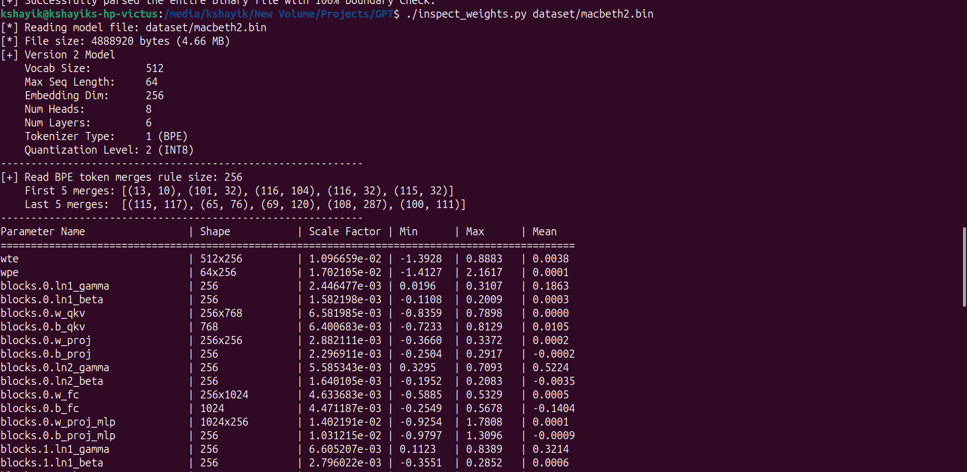
Matrix dimensions and blocks

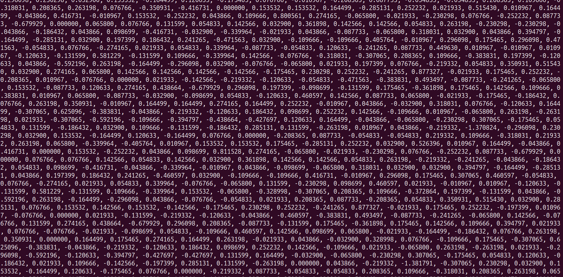
Raw model weights

This is only a ridiculously tiny fraction of the model. Our entire trained model contains roughly 4.66 MB of weights. The numbers you're looking at above are real weight values taken from the model — not some randomly generated example. But there's another interesting problem: those numbers don't necessarily have to stay as full-precision floating-point values.

Quantization

During quantization, we represent the same learned weights using fewer bits. Move the slider and watch what happens to the values. As the representation gets smaller, the weights require less storage, but we also lose numerical precision. For example, a value like 0.384721 might eventually be represented by a much smaller integer value such as 49, with a scale used to map between the two representations.

The slider above makes that trade-off visible. We're taking the same underlying weights and progressively reducing the amount of information used to represent them. And that trade-off is exactly what makes the next experiment possible: our model took hours to train, but after quantization its weight payload is only around 4.66 MB. Now let's see whether we can somehow cram that entire thing into an ESP32.

The Absurd Finale: Squeezing GPT onto an ESP32

After building a model that needs hours of computation to train, I wanted to take it in the complete opposite direction.

How small can we make it?

Our trained model features 6 Transformer layers, 256-dimensional embeddings, 8 attention heads, and a 512-token BPE vocabulary. The underlying architecture and learned weights remain the same; what changes is the numerical representation (quantized to 8-bit INT8) and the runtime used to execute them. By stripping out dynamic heap allocations in favor of a single pre-allocated scratchpad and reading our ~4.66 MB weight payload directly out of memory-mapped Flash ROM, we force an entire autoregressive Transformer to run inside 520 KB of internal SRAM.

That's small enough to make the next experiment possible. We're taking the trained weights and putting them on an ESP32 — a tiny dual-core microcontroller with roughly 520 KB of internal SRAM.

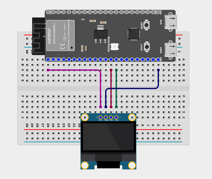
Circuit schematic: ESP32-S3 connected to a SSD1306 OLED display via I2C

Obviously, we can't just dump the entire model into RAM and call it a day. The weights live in Flash, while the activations are handled through carefully managed buffers in RAM. Instead of constantly allocating and freeing memory during generation, the runtime uses pre-allocated buffers and reuses them throughout the forward pass. The model itself doesn't suddenly become different. The same embeddings, attention, LayerNorm, feed-forward layers and autoregressive generation are still happening. We're just forcing all of it through a machine that was never designed to run a Transformer.

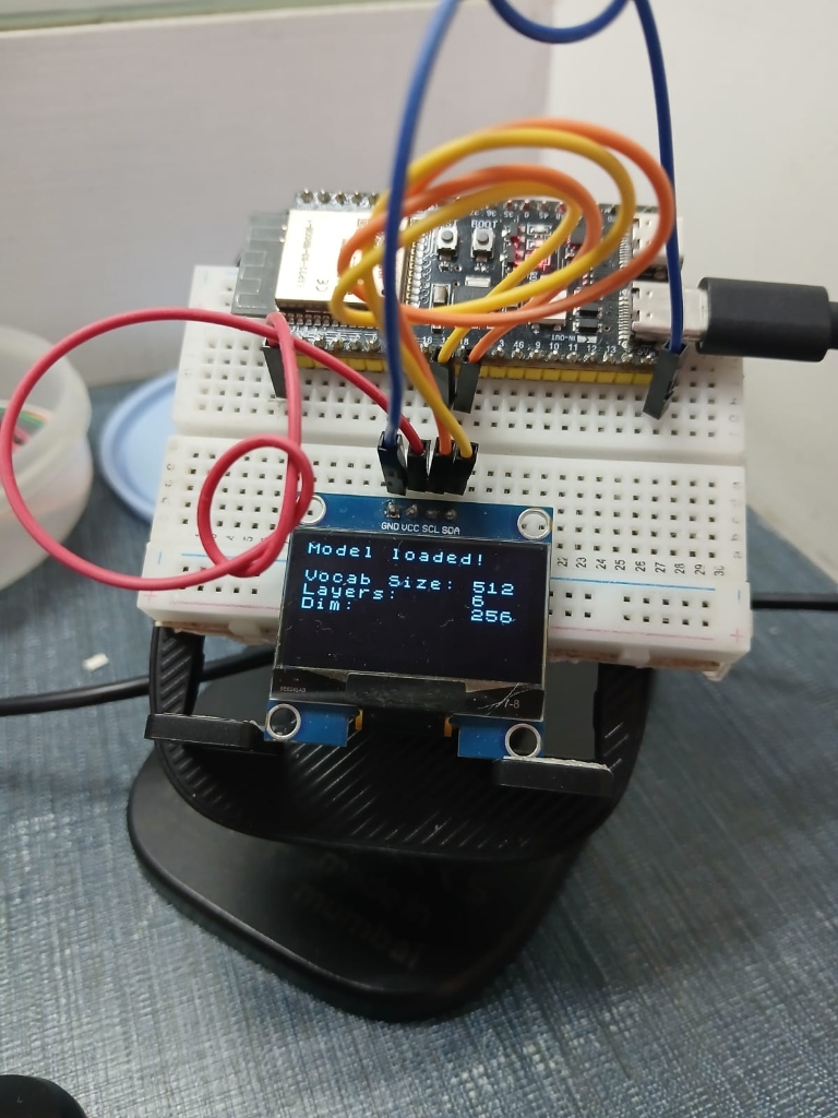
And that's probably the best place to end this series.

Full Circle

Look at where we started.

• Part 1: Tokens, context, tensors and next-token prediction.
• Part 2: Attention, QKV, masking, multi-head attention and the Transformer block.
• Part 3: Took those equations and rebuilt them in C++, then squeezed the CPU with contiguous memory, AVX2, FMA and OpenMP.
• Part 4: Went down another level — into GPU architecture, CUDA, parallel execution and memory hierarchies — and then took the finished model all the way down to an ESP32.

The interesting part isn't that we built a tiny GPT. It's that we followed the same computation through almost the entire stack:

Mathematics → C++ → CPU → GPU → embedded silicon

We didn't just build the model. We opened the black box.

The series is complete. Thank you for reading! 🚀

If you ended up building your own Transformer, optimizing something differently, or spotting a bug in my implementation, I'd genuinely love to hear about it. The complete project is open source: GitHub Repository ↗