From Whiteboard to C++

If you've made it this far, welcome to the real work. In Part 1, we covered the tokenization, sequence chunking, and foundational math. In Part 2, we dissected the Query-Key-Value (QKV) self-attention engine, multi-head attention, layer normalization, and feed-forward blocks. Now, it's time to take all those whiteboard equations and translate them into modern, raw C++.

As we move ahead, you might need this. Keep it handy.

Over the last two articles, we understood how GPT works mathematically. Today, we're finally going to build it.

Before writing a single line of code, though, I want you all to answer one question: Can you execute an entire GPT forward pass with nothing but a notebook, a pen, and a calculator?

It sounds absurd, but I genuinely encourage you to try it before you print "Hello world" 😋

So... I sat down and deliberately built the smallest possible GPT by hand. Every embedding lookup, every attention score, every LayerNorm, every FFN output, and finally the vocabulary probabilities were computed manually. In other words, the complete forward pass, from the input tokens all the way to the final predicted token. It completely changed how I thought about implementing Transformers.

I've attached the complete handwritten derivation below if you'd like to follow along.

I also made this tensor transformation blueprint while studying. It became my reference point throughout the implementation.

The complete source code is available if you'd like to follow along.

You could cheat and peek at the implementation right now... 😏
But I'd recommend staying with me until the end. Building it yourself teaches you far more than reading my code ever will.

A Small Note

I won't be going through the implementation line by line. Personally, I think that kills creativity. There are ten different ways to write the exact same piece of code, and I want you to write your version instead of copying mine. Think of this article as a set of directions and engineering notes based on my own journey, not a tutorial to copy and paste.

1. Matrices Are a Myth

One of the biggest misconceptions I had before implementing GPT was how tensors are actually stored in memory. Whenever we draw matrices on paper, we naturally imagine that computers store them exactly the same way: neat rows and columns, stacked together into 3D blocks.

Something like this:

// Multi-dimensional nested vectors 

std::vector<std::vector<std::vector<float>>> tensor;

// Or raw 3D array 

float tensor[B][T][C];

After all, as we learned earlier, a Transformer constantly works with tensors shaped like: $[B \times T \times C ]$

So using nested vectors almost feels... obvious. Unfortunately, it's also one of the slowest ways to represent a tensor.

Why Nested Vectors Become a Performance Nightmare

To understand why, we first need to understand how a std::vector actually stores its data.

Every std::vector owns its own heap allocation. A three-dimensional vector therefore isn't one giant block of memory. Instead, it becomes hundreds or even thousands of tiny allocations pointing to one another.

Visually, we imagine something like this:

[B]
 ├── [T]
 │     ├── [C]
 │     ├── [C]
 │     └── [C]
 │
 ├── [T]
 │     ├── [C]
 │     └── [C]

Every level introduces another pointer dereference. Every sub-vector may live in a completely different region of memory. When matrix multiplication begins, the processor spends an alarming amount of time chasing pointers instead of doing the actual math.

Cache Misses: The Hidden Enemy

Modern CPUs are unbelievably fast. But the RAM isn't.

To hide that latency, CPUs keep recently accessed data inside tiny but incredibly fast caches. These caches work best when memory is contiguous. Nested vectors completely destroy this advantage. Instead of reading memory sequentially, pointer-chasing forces the CPU to jump non-contiguously, stalling while fetching new memory lines:

For neural networks performing billions of floating-point operations, those waits quickly become one of the biggest performance bottlenecks.

Thinking Like TensorFlow

This completely changed the way I thought about tensors. Frameworks like PyTorch and TensorFlow don't store tensors as nested containers. They store them as one giant contiguous block of memory.

Something much closer to:

std::vector<float> data;
std::vector<size_t> shape;
std::vector<size_t> strides;

That's genuinely it.

Internally, this still represents a tensor of shape $[ B \times T \times C ]$.
The only difference is that the dimensions become metadata rather than nested containers.

So... How Do We Find an Element?

This was the next question I had. If everything is flattened into one long array, how do we access $X[b][t][c]$ without actually having three dimensions?

The answer is surprisingly elegant. Every dimension is assigned a stride, telling us how many elements we need to skip in memory before moving one step along that axis. For a contiguous tensor:

which gives us the flat memory index:

That's it. One arithmetic expression is enough to locate any element inside a three-dimensional tensor. Once I understood this, tensors stopped feeling like mysterious AI objects. They became exactly what they really are: a flat chunk of memory with a bit of metadata attached to it.

2. Translating Mathematics into Objects

After establishing how flat tensors live in contiguous memory, the next challenge was translating theoretical research equations into reusable C++ objects.

On paper, every Transformer layer is just a single line of linear algebra. In code, however, each equation becomes an independent module responsible for one specific state transformation. Instead of writing one giant, monolithic function, I broke the model into modular building blocks. Each class owns its learnable parameters, executes its specific mathematical operation, and passes the transformed tensor to the next stage.

Once these pieces existed independently, assembling the Transformer became surprisingly clean.

Token & Positional Embeddings

The input to GPT is simply a matrix of integer token IDs. The model's very first job is converting those discrete integers into dense, continuous vector representations.

Mathematically, this is just a combined lookup from the Token Embedding table $W_{te} \in \mathbb{R}^{V \times C}$ and the Positional Embedding table $W_{pe} \in \mathbb{R}^{T \times C}$:

Rather than allocating two intermediate tensors and adding them afterward, I combined both lookups directly inside the embedding loop, writing the final sum straight into the output tensor.

One small but crucial lesson I learned writing low-level C++ was how valuable assert becomes. Unlike Python, an invalid index won't always throw a friendly exception. Sometimes it happily reads garbage memory and lets your network quietly produce numerical nonsense. Adding assertions around tensor boundaries saved me hours of head-scratching debugging.

Layer Normalization

LayerNorm was probably the first component where the C++ implementation looked noticeably longer than the equation itself. The mathematics is beautifully compact:

Implementing it, however, means computing the mean, variance, normalization, and learnable scale and shift parameters for every token independently across the channel dimension.

One funny thing I noticed while solving GPT manually on paper was how LayerNorm behaves when the embedding dimension is tiny. For my handwritten walkthrough, I intentionally chose $C = 2$ to keep the arithmetic manageable. LayerNorm almost behaved like a sign operator, pushing values strictly to $[-1, 1]$. Of course, production models like GPT-2 use $C = 768$, where LayerNorm estimates much smoother feature statistics across hundreds of active channels.

Masked Multi-Head Self-Attention

This is where the code finally started feeling like "real GPT." The pipeline follows the mathematics almost one-to-one:

1. Project the normalized input into Query ($Q$), Key ($K$), and Value ($V$) matrices.
2. Compute scaled dot-product attention scores using $\frac{Q K^T}{\sqrt{d_k}}$.
3. Apply the causal mask by setting upper-triangular elements to $-infty$ so future tokens receive exact zero attention after Softmax.
4. Multiply the resulting attention weights by the Value matrix to yield contextual embeddings.

The equations themselves are elegant, but translating them into C++ was where the real engineering began—managing matrix multiplications, tensor reshapes, head splitting, row-wise Softmax, and careful stride indexing over flat memory.

Feed-Forward Network

Once attention finishes exchanging information between tokens, each token is processed independently by a position-wise feed-forward network. Architecturally, the feature dimension expands from $C \to 4C$, passes through a non-linear activation, and projects back down from $4C o C$.

I chose GELU (Gaussian Error Linear Unit) over standard ReLU because it provides a smooth, non-zero gradient response for negative inputs near zero. Modern GPT models rely heavily on this subtle architectural detail to maintain stable gradient flow during deep network training.

3. Assembling the Transformer

At this point, every mathematical building block existed independently: Embedding, LayerNorm, CausalSelfAttention, and FeedForward. Now came the most satisfying part: plugging everything together.

One of the most important architectural choices I made was using Pre-LayerNorm, matching modern GPT models. Instead of normalizing after each sub-layer, the input vector is normalized first:

The residual skip connection acts like an unblocked gradient highway, allowing information to flow through the network without being constantly distorted. As Transformer models stack deeper, these residual connections are the primary reason training stays numerically stable.

Once a single Transformer block was working, the top-level architecture became clean and modular—the output of one block simply becomes the input to the next:

After the final block, one last LayerNorm is applied before projecting every token back into vocabulary space through the Language Model Head. Mathematically, this is another matrix multiplication:

where $W_{lm} \in \mathbb{R}^{C \times V}$. Applying a row-wise Softmax over these logits yields a probability distribution over the entire vocabulary, allowing GPT to sample the next predicted token.

Watching GPT Learn

Now, while the model is busy training, I'd like to loop back to something. If you've been following this series from the beginning, you might remember the output from Part 1. Back then, our tiny Bigram model generated... well... pure AI gibberish:

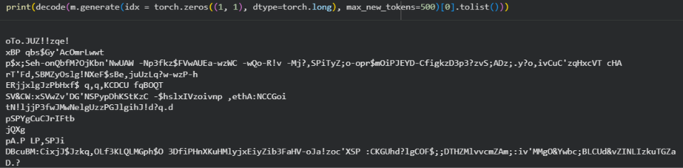
Before training: The raw Bigram output from Part 1.

Now, after training is completed, I present to you Chat GPT from TEMU:

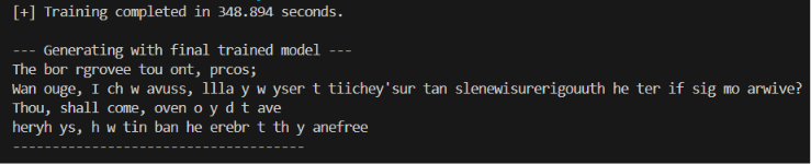
After training: Shakespeare-like text structure emerges.

Reading:

"Thou, shall come, oven o y d t ave
heryh ys, h w tin ban he erebr t th y anefree"

for the first time genuinely made me smile. Remember what we're training here. This is only a 4-layer Transformer with an embedding dimension of 128, 4 attention heads, trained entirely on a CPU with a tiny parameter count and only a few hundred optimization steps. We're nowhere near GPT-2 or GPT-3 territory. But that was never the goal.

And now that we know it works... We have another problem :(

4. It Worked... Now It Had to Become Fast

The first successful forward pass felt incredible. The first benchmark did not.

Everything was mathematically exact, but execution was painfully sluggish. Most of the runtime wasn't even spent doing heavy arithmetic. It was spent moving data around memory.

That realization completely shifted my approach to optimization. Instead of asking "How can I make matrix multiplication faster?", I started asking

"How can I make the CPU touch memory less?"

The first fix was already built into our foundation: replacing nested vectors with flat, contiguous memory. From there, the gains became deeply hardware-focused:

• Cache Locality: Reordering matrix multiplication loops so access patterns walk linearly through contiguous memory rows rather than jumping down memory columns.
• SIMD Vectorization: Leveraging 256-bit AVX2 registers and Fused Multiply-Add (FMA) instructions to execute multiple 32-bit floating-point operations in a single CPU instruction cycle.
• OpenMP Parallelism: Adding multithreading pragmas across independent batch and attention-head loops to distribute workload across all available CPU cores with zero changes to the underlying math.

None of these tweaks altered the underlying equations. The math stayed identical—only the execution efficiency changed. Building a Transformer isn't just about attention or linear algebra; it's about understanding memory, CPU cache lines, and hardware execution. The paper tells you what to compute; good engineering decides how fast you get there.

Measuring the Improvements

Of course, saying something became "faster" doesn't really mean much unless you can measure it.

Thankfully, Linux gives us exactly the tool for that. The perf utility lets us inspect hardware performance counters exposed directly by the CPU, making it possible to measure things like cache misses, branch prediction, CPU cycles, and much more.
For this project, I focused on cache behavior using:

perf stat -e cache-misses,L1-dcache-load-misses ./build/engine

After applying the optimizations, the total execution time dropped from roughly 350 seconds to just under 283 seconds.

Here's the overall comparison:

And here's the actual perf output collected from the optimized implementation:

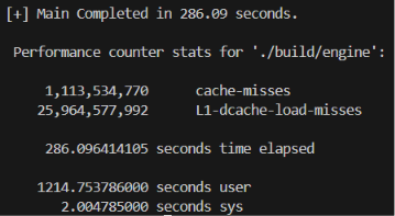
Linux perf output: 1.11B cache misses and 286 seconds elapsed time.

For me, the most satisfying metric wasn't even the reduction in execution time. It was seeing nearly 300 million fewer cache misses. That was a direct confirmation that the changes to memory layout and access patterns were actually helping the CPU spend less time waiting on RAM and more time doing useful work.

Looking Ahead

Throughout this project, I intentionally kept the model small enough to train comfortably on a CPU. The implementation you've seen uses:

• 4 Transformer layers
• Embedding Dimension = 128
• 4 Attention Heads
• Character-level vocabulary (65 tokens)

This configuration is perfect for understanding the architecture, debugging tensor transformations, and validating the implementation.

Modern language models operate on an entirely different scale. GPT-2 Small already uses 12 layers, 768-dimensional embeddings, and 124 million parameters. Today's frontier models, such as GPT-4 or Gemini, are believed to contain hundreds of billions to even trillions of parameters, trained across thousands of GPUs over weeks or even months. While the exact architectures aren't public, they're several orders of magnitude larger than the implementation we've built here.

At that scale, CPU optimization alone simply isn't enough. The next step is moving the exact same implementation onto the GPU.

In the final part of this series, we'll explore CUDA, GPU kernels, and parallel matrix multiplication to understand why modern Transformers simply wouldn't exist without GPU acceleration.

See you in Part 4. 🚀

If you ended up building your own Transformer, optimizing something differently, or spotting a bug in my implementation, I'd genuinely love to hear about it. The complete project is open source: GitHub Repository ↗